3. Tutorial

This tutorial will guide you through a typical PyMC application. Familiarity with Python is assumed, so if you are new to Python, books such as [Lutz2007] or [Langtangen2009] are the place to start. Plenty of online documentation can also be found on the Python documentation page.

3.1. An example statistical model

Consider the following dataset, which is a time series of recorded coal mining disasters in the UK from 1851 to 1962 [Jarrett1979].

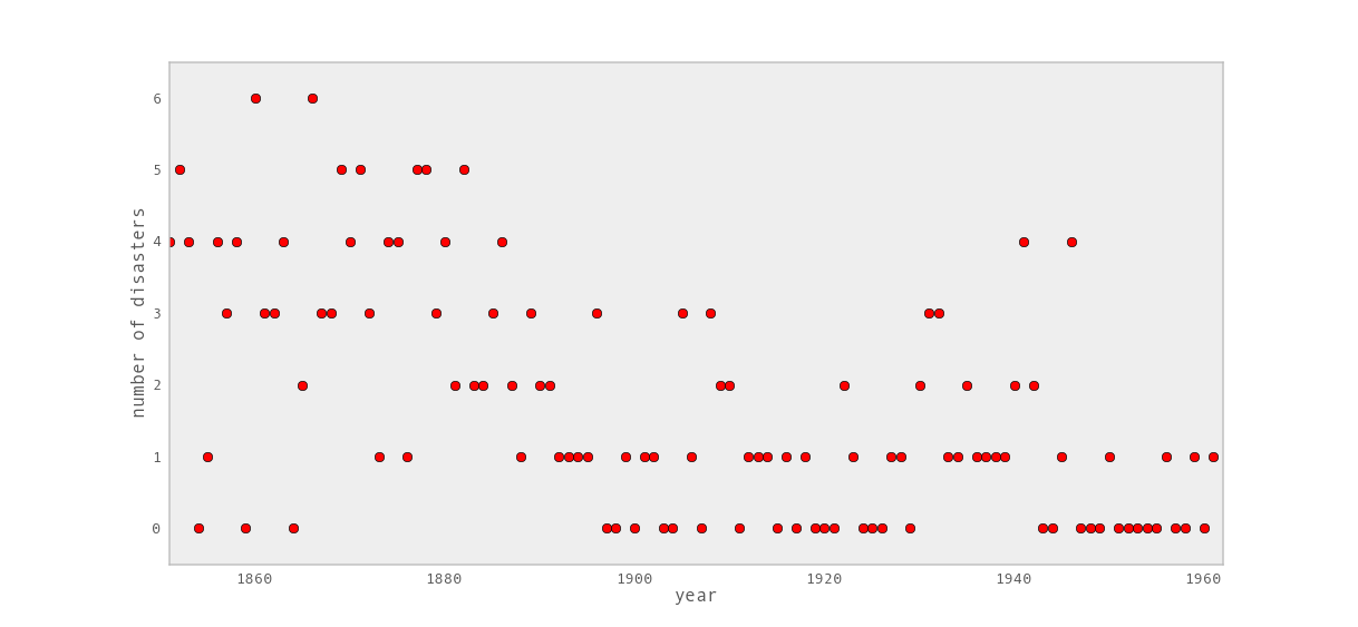
Recorded coal mining disasters in the UK.

Occurrences of disasters in the time series is thought to be derived from a Poisson process with a large rate parameter in the early part of the time series, and from one with a smaller rate in the later part. We are interested in locating the change point in the series, which perhaps is related to changes in mining safety regulations.

We represent our conceptual model formally as a statistical model:

\[\begin{split}\begin{array}{ccc} (D_t | s, e, l) \sim\text{Poisson}\left(r_t\right), & r_t=\left\{\begin{array}{lll} e &\text{if}& t< s\\ l &\text{if}& t\ge s \end{array}\right.,&t\in[t_l,t_h]\\ s\sim \text{Discrete Uniform}(t_l, t_h)\\ e\sim \text{Exponential}(r_e)\\ l\sim \text{Exponential}(r_l) \end{array}\end{split}\]

The symbols are defined as:

• \(D_t\): The number of disasters in year \(t\).
• \(r_t\): The rate parameter of the Poisson distribution of disasters in year \(t\).
• \(s\): The year in which the rate parameter changes (the switchpoint).
• \(e\): The rate parameter before the switchpoint \(s\).
• \(l\): The rate parameter after the switchpoint \(s\).
• \(t_l\), \(t_h\): The lower and upper boundaries of year \(t\).
• \(r_e\), \(r_l\): The rate parameters of the priors of the early and late rates, respectively.

Because we have defined \(D\) by its dependence on \(s\), \(e\) and \(l\), the latter three are known as the “parents” of \(D\) and \(D\) is called their “child”. Similarly, the parents of \(s\) are \(t_l\) and \(t_h\), and \(s\) is the child of \(t_l\) and \(t_h\).

3.2. Two types of variables

At the model-specification stage (before the data are observed), \(D\), \(s\), \(e\), \(r\) and \(l\) are all random variables. Bayesian “random” variables have not necessarily arisen from a physical random process. The Bayesian interpretation of probability is epistemic, meaning random variable \(x\)‘s probability distribution \(p(x)\) represents our knowledge and uncertainty about \(x\)‘s value [Jaynes2003]. Candidate values of \(x\) for which \(p(x)\) is high are relatively more probable, given what we know. Random variables are represented in PyMC by the classes Stochastic and Deterministic.

The only Deterministic in the model is \(r\). If we knew the values of \(r\)‘s parents (\(s\), \(l\) and \(e\)), we could compute the value of \(r\) exactly. A Deterministic like \(r\) is defined by a mathematical function that returns its value given values for its parents. Deterministic variables are sometimes called the systemic part of the model. The nomenclature is a bit confusing, because these objects usually represent random variables; since the parents of \(r\) are random, \(r\) is random also. A more descriptive (though more awkward) name for this class would be DeterminedByValuesOfParents.

On the other hand, even if the values of the parents of variables switchpoint, disasters (before observing the data), early_mean or late_mean were known, we would still be uncertain of their values. These variables are characterized by probability distributions that express how plausible their candidate values are, given values for their parents. The Stochastic class represents these variables. A more descriptive name for these objects might be RandomEvenGivenValuesOfParents.

We can represent model disaster_model in a file called disaster_model.py (the actual file can be found in pymc/examples/) as follows. First, we import the PyMC and NumPy namespaces:

from pymc import DiscreteUniform, Exponential, deterministic, Poisson, Uniform
import numpy as np

Notice that from pymc we have only imported a select few objects that are needed for this particular model, whereas the entire numpy namespace has been imported, and conveniently given a shorter name. Objects from NumPy are subsequently accessed by prefixing np. to the name. Either approach is acceptable.

Next, we enter the actual data values into an array:

disasters_array =   \
     np.array([ 4, 5, 4, 0, 1, 4, 3, 4, 0, 6, 3, 3, 4, 0, 2, 6,
                   3, 3, 5, 4, 5, 3, 1, 4, 4, 1, 5, 5, 3, 4, 2, 5,
                   2, 2, 3, 4, 2, 1, 3, 2, 2, 1, 1, 1, 1, 3, 0, 0,
                   1, 0, 1, 1, 0, 0, 3, 1, 0, 3, 2, 2, 0, 1, 1, 1,
                   0, 1, 0, 1, 0, 0, 0, 2, 1, 0, 0, 0, 1, 1, 0, 2,
                   3, 3, 1, 1, 2, 1, 1, 1, 1, 2, 4, 2, 0, 0, 1, 4,
                   0, 0, 0, 1, 0, 0, 0, 0, 0, 1, 0, 0, 1, 0, 1])

Note that you don’t have to type in this entire array to follow along; the code is available in the source tree, in this example script. Next, we create the switchpoint variable switchpoint

switchpoint = DiscreteUniform('switchpoint', lower=0, upper=110, doc='Switchpoint[year]')

DiscreteUniform is a subclass of Stochastic that represents uniformly-distributed discrete variables. Use of this distribution suggests that we have no preference a priori regarding the location of the switchpoint; all values are equally likely. Now we create the exponentially-distributed variables early_mean and late_mean for the early and late Poisson rates, respectively:

early_mean = Exponential('early_mean', beta=1.)
late_mean = Exponential('late_mean', beta=1.)

Next, we define the variable rate, which selects the early rate early_mean for times before switchpoint and the late rate late_mean for times after switchpoint. We create rate using the deterministic decorator, which converts the ordinary Python function rate into a Deterministic object.:

@deterministic(plot=False)
def rate(s=switchpoint, e=early_mean, l=late_mean):
    ''' Concatenate Poisson means '''
    out = np.empty(len(disasters_array))
    out[:s] = e
    out[s:] = l
    return out

The last step is to define the number of disasters disasters. This is a stochastic variable but unlike switchpoint, early_mean and late_mean we have observed its value. To express this, we set the argument observed to True (it is set to False by default). This tells PyMC that this object’s value should not be changed:

disasters = Poisson('disasters', mu=rate, value=disasters_array, observed=True)

3.2.1. Why are data and unknown variables represented by the same object?

Since its represented by a Stochastic object, disasters is defined by its dependence on its parent rate even though its value is fixed. This isn’t just a quirk of PyMC’s syntax; Bayesian hierarchical notation itself makes no distinction between random variables and data. The reason is simple: to use Bayes’ theorem to compute the posterior \(p(e,s,l \mid D)\) of model disaster_model, we require the likelihood \(p(D \mid e,s,l)\). Even though disasters‘s value is known and fixed, we need to formally assign it a probability distribution as if it were a random variable. Remember, the likelihood and the probability function are essentially the same, except that the former is regarded as a function of the parameters and the latter as a function of the data.

This point can be counterintuitive at first, as many peoples’ instinct is to regard data as fixed a priori and unknown variables as dependent on the data. One way to understand this is to think of statistical models like disaster_model as predictive models for data, or as models of the processes that gave rise to data. Before observing the value of disasters, we could have sampled from its prior predictive distribution \(p(D)\) (i.e. the marginal distribution of the data) as follows:

• Sample early_mean, switchpoint and late_mean from their priors.
• Sample disasters conditional on these values.

Even after we observe the value of disasters, we need to use this process model to make inferences about early_mean , switchpoint and late_mean because it’s the only information we have about how the variables are related.

3.3. Parents and children

We have above created a PyMC probability model, which is simply a linked collection of variables. To see the nature of the links, import or run disaster_model.py and examine switchpoint‘s parents attribute from the Python prompt:

>>> from pymc.examples import disaster_model
>>> disaster_model.switchpoint.parents
{'lower': 0, 'upper': 110}

The parents dictionary shows us the distributional parameters of switchpoint, which are constants. Now let’s examine disasters‘s parents:

>>> disaster_model.disasters.parents
{'mu': <pymc.PyMCObjects.Deterministic 'rate' at 0x10623da50>}

We are using rate as a distributional parameter of disasters (i.e. rate is disasters‘s parent). disasters internally labels rate as mu, meaning rate plays the role of the rate parameter in disasters‘s Poisson distribution. Now examine rate‘s children attribute:

>>> disaster_model.rate.children
set([<pymc.distributions.Poisson 'disasters' at 0x10623da90>])

Because disasters considers rate its parent, rate considers disasters its child. Unlike parents, children is a set (an unordered collection of objects); variables do not associate their children with any particular distributional role. Try examining the parents and children attributes of the other parameters in the model.

The following directed acyclic graph is a visualization of the parent-child relationships in the model. Unobserved stochastic variables switchpoint, early_mean and late_mean are open ellipses, observed stochastic variable disasters is a filled ellipse and deterministic variable rate is a triangle. Arrows point from parent to child and display the label that the child assigns to the parent. See section Graphing models for more details.

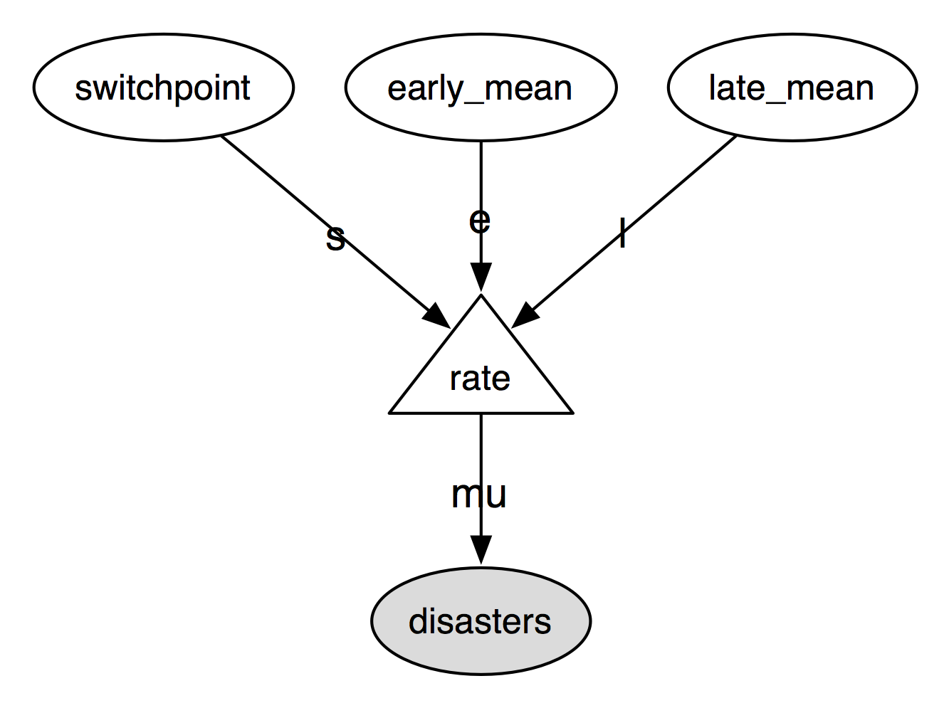
Directed acyclic graph of the relationships in the coal mining disaster model example.

As the examples above have shown, pymc objects need to have a name assigned, such as switchpoint, early_mean or late_mean. These names are used for storage and post-processing:

• as keys in on-disk databases,
• as node labels in model graphs,
• as axis labels in plots of traces,
• as table labels in summary statistics.

A model instantiated with variables having identical names raises an error to avoid name conflicts in the database storing the traces. In general however, pymc uses references to the objects themselves, not their names, to identify variables.

3.4. Variables’ values and log-probabilities

All PyMC variables have an attribute called value that stores the current value of that variable. Try examining disasters‘s value, and you’ll see the initial value we provided for it:

>>> disaster_model.disasters.value
array([4, 5, 4, 0, 1, 4, 3, 4, 0, 6, 3, 3, 4, 0, 2, 6, 3, 3, 5, 4, 5, 3, 1,
       4, 4, 1, 5, 5, 3, 4, 2, 5, 2, 2, 3, 4, 2, 1, 3, 2, 2, 1, 1, 1, 1, 3,
       0, 0, 1, 0, 1, 1, 0, 0, 3, 1, 0, 3, 2, 2, 0, 1, 1, 1, 0, 1, 0, 1, 0,
       0, 0, 2, 1, 0, 0, 0, 1, 1, 0, 2, 3, 3, 1, 1, 2, 1, 1, 1, 1, 2, 4, 2,
       0, 0, 1, 4, 0, 0, 0, 1, 0, 0, 0, 0, 0, 1, 0, 0, 1, 0, 1])

If you check the values of early_mean, switchpoint and late_mean, you’ll see random initial values generated by PyMC:

>>> disaster_model.switchpoint.value
44

>>> disaster_model.early_mean.value
0.33464706250079584

>>> disaster_model.late_mean.value
2.6491936762267811

Of course, since these are Stochastic elements, your values will be different than these. If you check rate‘s value, you’ll see an array whose first switchpoint elements are early_mean (here 0.33464706), and whose remaining elements are late_mean (here 2.64919368):

>>> disaster_model.rate.value
array([ 0.33464706,  0.33464706,  0.33464706,  0.33464706,  0.33464706,
        0.33464706,  0.33464706,  0.33464706,  0.33464706,  0.33464706,
        0.33464706,  0.33464706,  0.33464706,  0.33464706,  0.33464706,
        0.33464706,  0.33464706,  0.33464706,  0.33464706,  0.33464706,
        0.33464706,  0.33464706,  0.33464706,  0.33464706,  0.33464706,
        0.33464706,  0.33464706,  0.33464706,  0.33464706,  0.33464706,
        0.33464706,  0.33464706,  0.33464706,  0.33464706,  0.33464706,
        0.33464706,  0.33464706,  0.33464706,  0.33464706,  0.33464706,
        0.33464706,  0.33464706,  0.33464706,  0.33464706,  2.64919368,
        2.64919368,  2.64919368,  2.64919368,  2.64919368,  2.64919368,
        2.64919368,  2.64919368,  2.64919368,  2.64919368,  2.64919368,
        2.64919368,  2.64919368,  2.64919368,  2.64919368,  2.64919368,
        2.64919368,  2.64919368,  2.64919368,  2.64919368,  2.64919368,
        2.64919368,  2.64919368,  2.64919368,  2.64919368,  2.64919368,
        2.64919368,  2.64919368,  2.64919368,  2.64919368,  2.64919368,
        2.64919368,  2.64919368,  2.64919368,  2.64919368,  2.64919368,
        2.64919368,  2.64919368,  2.64919368,  2.64919368,  2.64919368,
        2.64919368,  2.64919368,  2.64919368,  2.64919368,  2.64919368,
        2.64919368,  2.64919368,  2.64919368,  2.64919368,  2.64919368,
        2.64919368,  2.64919368,  2.64919368,  2.64919368,  2.64919368,
        2.64919368,  2.64919368,  2.64919368,  2.64919368,  2.64919368,
        2.64919368,  2.64919368,  2.64919368,  2.64919368,  2.64919368])

To compute its value, rate calls the function we used to create it, passing in the values of its parents.

Stochastic objects can evaluate their probability mass or density functions at their current values given the values of their parents. The logarithm of a stochastic object’s probability mass or density can be accessed via the logp attribute. For vector-valued variables like disasters, the logp attribute returns the sum of the logarithms of the joint probability or density of all elements of the value. Try examining switchpoint‘s and disasters‘s log-probabilities and early_mean ‘s and late_mean‘s log-densities:

>>> disaster_model.switchpoint.logp
-4.7095302013123339

>>> disaster_model.disasters.logp
-1080.5149888046033

>>> disaster_model.early_mean.logp
-0.33464706250079584

>>> disaster_model.late_mean.logp
-2.6491936762267811

Stochastic objects need to call an internal function to compute their logp attributes, as rate needed to call an internal function to compute its value. Just as we created rate by decorating a function that computes its value, it’s possible to create custom Stochastic objects by decorating functions that compute their log-probabilities or densities (see chapter Building models). Users are thus not limited to the set of statistical distributions provided by PyMC.

3.4.1. Using Variables as parents of other Variables

Let’s take a closer look at our definition of rate:

@deterministic(plot=False)
def rate(s=switchpoint, e=early_mean, l=late_mean):
    ''' Concatenate Poisson means '''
    out = np.empty(len(disasters_array))
    out[:s] = e
    out[s:] = l
    return out

The arguments switchpoint, early_mean and late_mean are Stochastic objects, not numbers. If that is so, why aren’t errors raised when we attempt to slice array out up to a Stochastic object?

Whenever a variable is used as a parent for a child variable, PyMC replaces it with its value attribute when the child’s value or log-probability is computed. When rate‘s value is recomputed, s.value is passed to the function as argument switchpoint. To see the values of the parents of rate all together, look at rate.parents.value.

3.5. Fitting the model with MCMC

PyMC provides several objects that fit probability models (linked collections of variables) like ours. The primary such object, MCMC, fits models with a Markov chain Monte Carlo algorithm [Gamerman1997]. To create an MCMC object to handle our model, import disaster_model.py and use it as an argument for MCMC:

>>> from pymc.examples import disaster_model
>>> from pymc import MCMC
>>> M = MCMC(disaster_model)

In this case M will expose variables switchpoint, early_mean, late_mean and disasters as attributes; that is, M.switchpoint will be the same object as disaster_model.switchpoint.

To run the sampler, call the MCMC object’s sample() (or isample(), for interactive sampling) method with arguments for the number of iterations, burn-in length, and thinning interval (if desired):

>>> M.sample(iter=10000, burn=1000, thin=10)

After a few seconds, you should see that sampling has finished normally. The model has been fitted.

3.5.1. What does it mean to fit a model?

Fitting a model means characterizing its posterior distribution somehow. In this case, we are trying to represent the posterior \(p(s,e,l|D)\) by a set of joint samples from it. To produce these samples, the MCMC sampler randomly updates the values of switchpoint, early_mean and late_mean according to the Metropolis-Hastings algorithm [Gelman2004] over a specified number of iterations (iter).

As the number of samples grows sufficiently large, the MCMC distributions of switchpoint, early_mean and late_mean converge to their joint stationary distribution. In other words, their values can be considered as random draws from the posterior \(p(s,e,l|D)\). PyMC assumes that the burn parameter specifies a sufficiently large number of iterations for the algorithm to converge, so it is up to the user to verify that this is the case (see chapter Model checking and diagnostics). Consecutive values sampled from switchpoint, early_mean and late_mean are always serially dependent, since it is a Markov chain. MCMC often results in strong autocorrelation among samples that can result in imprecise posterior inference. To circumvent this, it is useful to thin the sample by only retaining every k th sample, where \(k\) is an integer value. This thinning interval is passed to the sampler via the thin argument.

If you are not sure ahead of time what values to choose for the burn and thin parameters, you may want to retain all the MCMC samples, that is to set burn=0 and thin=1, and then discard the burn-in period and thin the samples after examining the traces (the series of samples). See [Gelman2004] for general guidance.

3.5.2. Accessing the samples

The output of the MCMC algorithm is a trace, the sequence of retained samples for each variable in the model. These traces can be accessed using the trace(name, chain=-1) method. For example:

>>> M.trace('switchpoint')[:]
array([41, 40, 40, ..., 43, 44, 44])

The trace slice [start:stop:step] works just like the NumPy array slice. By default, the returned trace array contains the samples from the last call to sample, that is, chain=-1, but the trace from previous sampling runs can be retrieved by specifying the correspondent chain index. To return the trace from all chains, simply use chain=None. [2]

3.5.3. Sampling output

You can examine the marginal posterior of any variable by plotting a histogram of its trace:

>>> from pylab import hist, show
>>> hist(M.trace('late_mean')[:])
(array([   8,   52,  565, 1624, 2563, 2105, 1292,  488,  258,   45]),
 array([ 0.52721865,  0.60788251,  0.68854637,  0.76921023,  0.84987409,
        0.93053795,  1.01120181,  1.09186567,  1.17252953,  1.25319339]),
 <a list of 10 Patch objects>)
>>> show()

You should see something like this:

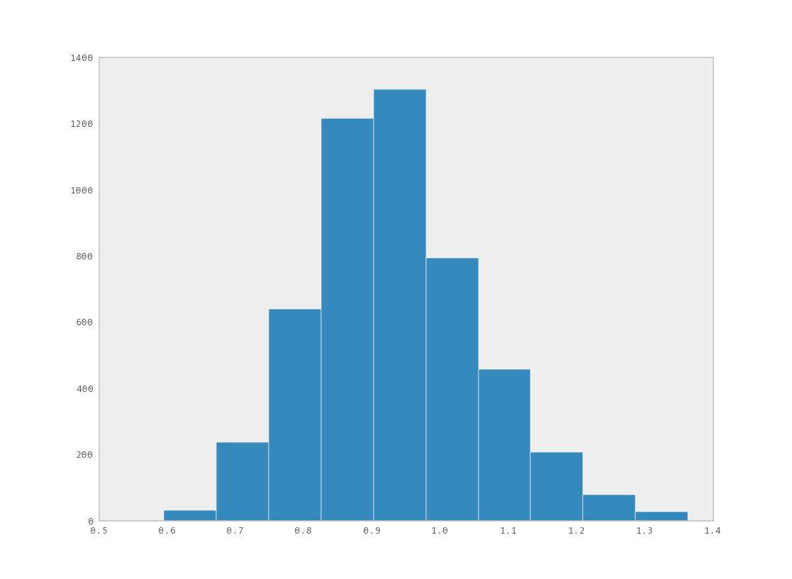
Histogram of the marginal posterior probability of parameter late_mean.

PyMC has its own plotting functionality, via the optional matplotlib module as noted in the installation notes. The Matplot module includes a plot function that takes the model (or a single parameter) as an argument:

>>> from pymc.Matplot import plot
>>> plot(M)

For each variable in the model, plot generates a composite figure, such as this one for the switchpoint in the disasters model:

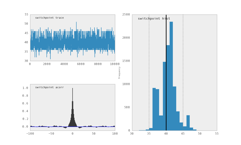
Temporal series, autocorrelation plot and histogram of the samples drawn for switchpoint.

The upper left-hand pane of this figure shows the temporal series of the samples from switchpoint, while below is an autocorrelation plot of the samples. The right-hand pane shows a histogram of the trace. The trace is useful for evaluating and diagnosing the algorithm’s performance (see [Gelman1996]), while the histogram is useful for visualizing the posterior.

For a non-graphical summary of the posterior, simply call M.stats().

3.5.4. Imputation of Missing Data

As with most textbook examples, the models we have examined so far assume that the associated data are complete. That is, there are no missing values corresponding to any observations in the dataset. However, many real-world datasets have missing observations, usually due to some logistical problem during the data collection process. The easiest way of dealing with observations that contain missing values is simply to exclude them from the analysis. However, this results in loss of information if an excluded observation contains valid values for other quantities, and can bias results. An alternative is to impute the missing values, based on information in the rest of the model.

For example, consider a survey dataset for some wildlife species:

Count	Site	Observer	Temperature
15	1	1	15
10	1	2	NA
6	1	1	11

Each row contains the number of individuals seen during the survey, along with three covariates: the site on which the survey was conducted, the observer that collected the data, and the temperature during the survey. If we are interested in modelling, say, population size as a function of the count and the associated covariates, it is difficult to accommodate the second observation because the temperature is missing (perhaps the thermometer was broken that day). Ignoring this observation will allow us to fit the model, but it wastes information that is contained in the other covariates.

In a Bayesian modelling framework, missing data are accommodated simply by treating them as unknown model parameters. Values for the missing data \(\tilde{y}\) are estimated naturally, using the posterior predictive distribution:

\[p(\tilde{y}|y) = \int p(\tilde{y}|\theta) f(\theta|y) d\theta\]

This describes additional data \(\tilde{y}\), which may either be considered unobserved data or potential future observations. We can use the posterior predictive distribution to model the likely values of missing data.

Consider the coal mining disasters data introduced previously. Assume that two years of data are missing from the time series; we indicate this in the data array by the use of an arbitrary placeholder value, None.:

x = np.array([ 4, 5, 4, 0, 1, 4, 3, 4, 0, 6, 3, 3, 4, 0, 2, 6,
3, 3, 5, 4, 5, 3, 1, 4, 4, 1, 5, 5, 3, 4, 2, 5,
2, 2, 3, 4, 2, 1, 3, None, 2, 1, 1, 1, 1, 3, 0, 0,
1, 0, 1, 1, 0, 0, 3, 1, 0, 3, 2, 2, 0, 1, 1, 1,
0, 1, 0, 1, 0, 0, 0, 2, 1, 0, 0, 0, 1, 1, 0, 2,
3, 3, 1, None, 2, 1, 1, 1, 1, 2, 4, 2, 0, 0, 1, 4,
0, 0, 0, 1, 0, 0, 0, 0, 0, 1, 0, 0, 1, 0, 1])

To estimate these values in PyMC, we generate a masked array. These are specialised NumPy arrays that contain a matching True or False value for each element to indicate if that value should be excluded from any computation. Masked arrays can be generated using NumPy’s ma.masked_equal function:

>>> masked_values = np.ma.masked_equal(x, value=None)
>>> masked_values
masked_array(data = [4 5 4 0 1 4 3 4 0 6 3 3 4 0 2 6 3 3 5 4 5 3 1 4 4 1 5 5 3
 4 2 5 2 2 3 4 2 1 3 -- 2 1 1 1 1 3 0 0 1 0 1 1 0 0 3 1 0 3 2 2 0 1 1 1 0 1 0
 1 0 0 0 2 1 0 0 0 1 1 0 2 3 3 1 -- 2 1 1 1 1 2 4 2 0 0 1 4 0 0 0 1 0 0 0 0 0 1
 0 0 1 0 1],
 mask = [False False False False False False False False False False False False
 False False False False False False False False False False False False
 False False False False False False False False False False False False
 False False False  True False False False False False False False False
 False False False False False False False False False False False False
 False False False False False False False False False False False False
 False False False False False False False False False False False  True
 False False False False False False False False False False False False
 False False False False False False False False False False False False
 False False False],
      fill_value=?)

This masked array, in turn, can then be passed to one of PyMC’s data stochastic variables, which recognizes the masked array and replaces the missing values with Stochastic variables of the desired type. For the coal mining disasters problem, recall that disaster events were modeled as Poisson variates:

>>> from pymc import Poisson
>>> disasters = Poisson('disasters', mu=rate, value=masked_values, observed=True)

Here rate is an array of means for each year of data, allocated according to the location of the switchpoint. Each element in disasters is a Poisson Stochastic, irrespective of whether the observation was missing or not. The difference is that actual observations are data Stochastics (observed=True), while the missing values are non-data Stochastics. The latter are considered unknown, rather than fixed, and therefore estimated by the MCMC algorithm, just as unknown model parameters.

The entire model looks very similar to the original model:

# Switchpoint
switch = DiscreteUniform('switch', lower=0, upper=110)
# Early mean
early_mean = Exponential('early_mean', beta=1)
# Late mean
late_mean = Exponential('late_mean', beta=1)

@deterministic(plot=False)
def rate(s=switch, e=early_mean, l=late_mean):
    """Allocate appropriate mean to time series"""
    out = np.empty(len(disasters_array))
    # Early mean prior to switchpoint
    out[:s] = e
    # Late mean following switchpoint
    out[s:] = l
    return out


# The inefficient way, using the Impute function:
# D = Impute('D', Poisson, disasters_array, mu=r)
#
# The efficient way, using masked arrays:
# Generate masked array. Where the mask is true,
# the value is taken as missing.
masked_values = masked_array(disasters_array, mask=disasters_array==-999)

# Pass masked array to data stochastic, and it does the right thing
disasters = Poisson('disasters', mu=rate, value=masked_values, observed=True)

Here, we have used the masked_array function, rather than masked_equal, and the value -999 as a placeholder for missing data. The result is the same.

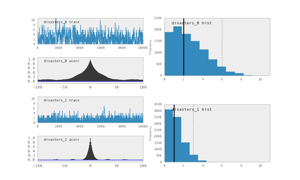
Trace, autocorrelation plot and posterior distribution of the missing data points in the example.

3.6. Fine-tuning the MCMC algorithm

MCMC objects handle individual variables via step methods, which determine how parameters are updated at each step of the MCMC algorithm. By default, step methods are automatically assigned to variables by PyMC. To see which step methods \(M\) is using, look at its step_method_dict attribute with respect to each parameter:

>>> M.step_method_dict[disaster_model.switchpoint]
[<pymc.StepMethods.DiscreteMetropolis object at 0x3e8cb50>]

>>> M.step_method_dict[disaster_model.early_mean]
[<pymc.StepMethods.Metropolis object at 0x3e8cbb0>]

>>> M.step_method_dict[disaster_model.late_mean]
[<pymc.StepMethods.Metropolis object at 0x3e8ccb0>]

The value of step_method_dict corresponding to a particular variable is a list of the step methods \(M\) is using to handle that variable.

You can force \(M\) to use a particular step method by calling M.use_step_method before telling it to sample. The following call will cause \(M\) to handle late_mean with a standard Metropolis step method, but with proposal standard deviation equal to \(2\):

>>> from pymc import Metropolis
>>> M.use_step_method(Metropolis, disaster_model.late_mean, proposal_sd=2.)

Another step method class, AdaptiveMetropolis, is better at handling highly-correlated variables. If your model mixes poorly, using AdaptiveMetropolis is a sensible first thing to try.

3.7. Beyond the basics

That was a brief introduction to basic PyMC usage. Many more topics are covered in the subsequent sections, including:

• Class Potential, another building block for probability models in addition to Stochastic and Deterministic
• Normal approximations
• Using custom probability distributions
• Object architecture
• Saving traces to the disk, or streaming them to the disk during sampling
• Writing your own step methods and fitting algorithms.

Also, be sure to check out the documentation for the Gaussian process extension, which is available on PyMC’s download page.

[2]	Note that the unknown variables switchpoint, early_mean,

late_mean and rate will all accrue samples, but disasters will not because its value has been observed and is not updated. Hence disasters has no trace and calling M.trace('disasters')[:] will raise an error.